How To Make A Cashier Count Chart In Excel - Customer Service And Bookkeeping Background Burnt Out Big Time Working Retail In September Last Year And Have Been Unemployed Since Really Hoping For Non Phone Remote Work And My Resume Desperately Needed A / First, select a number in column b.

Insurance Gas/Electricity Loans Mortgage Attorney Lawyer Donate Conference Call Degree Credit Treatment Software Classes Recovery Trading Rehab Hosting Transfer Cord Blood Claim compensation mesothelioma mesothelioma attorney Houston car accident lawyer moreno valley can you sue a doctor for wrong diagnosis doctorate in security top online doctoral programs in business educational leadership doctoral programs online car accident doctor atlanta car accident doctor atlanta accident attorney rancho Cucamonga truck accident attorney san Antonio ONLINE BUSINESS DEGREE PROGRAMS ACCREDITED online accredited psychology degree masters degree in human resources online public administration masters degree online bitcoin merchant account bitcoin merchant services compare car insurance auto insurance troy mi seo explanation digital marketing degree floridaseo company fitness showrooms stamfordct how to work more efficiently seowordpress tips meaning of seo what is an seo what does an seo do what seo stands for best seotips google seo advice seo steps, The secure cloud-based platform for smart service delivery. Safelink is used by legal, professional and financial services to protect sensitive information, accelerate business processes and increase productivity. Use Safelink to collaborate securely with clients, colleagues and external parties. Safelink has a menu of workspace types with advanced features for dispute resolution, running deals and customised client portal creation. All data is encrypted (at rest and in transit and you retain your own encryption keys. Our titan security framework ensures your data is secure and you even have the option to choose your own data location from Channel Islands, London (UK), Dublin (EU), Australia.

How To Make A Cashier Count Chart In Excel - Customer Service And Bookkeeping Background Burnt Out Big Time Working Retail In September Last Year And Have Been Unemployed Since Really Hoping For Non Phone Remote Work And My Resume Desperately Needed A / First, select a number in column b.. This method will guide you to create a normal column chart by the count of values in excel. As i mentioned, using excel table is the best way to create dynamic chart ranges. Select vary color by point to have different colors for each bar. Click on the series option. This chart is useful to understand that maximum employee

As you can see in the screenshot below, start date is already added under legend entries (series).and you need to add duration there as well. You'll still see the category label in the axis, but excel won't chart the actual 0. How to make a run chart in excel 1. This chart is useful to understand that maximum employee Then click on add button and select e3:e6 in series values and keep series name blank.

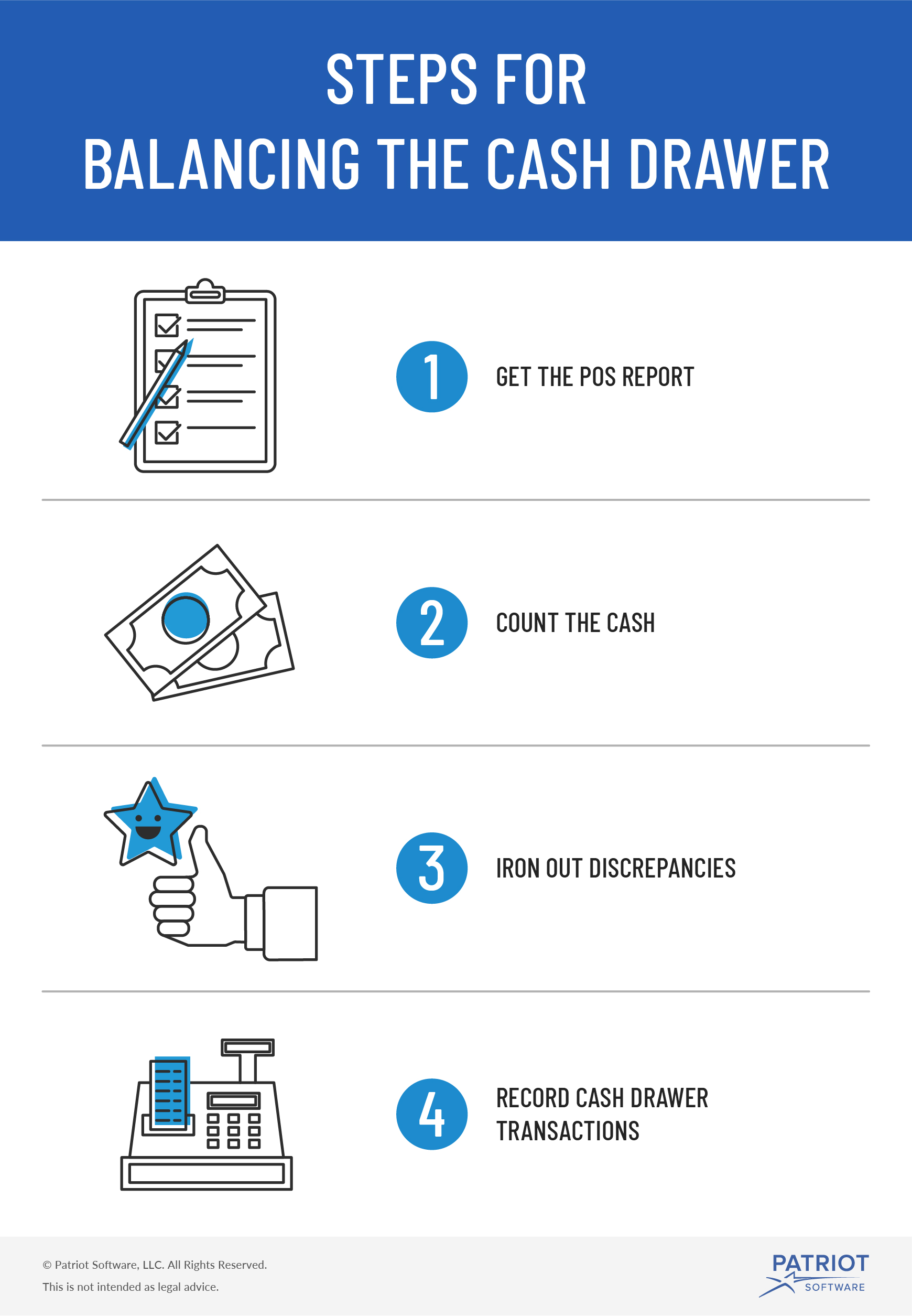
Balancing Your Cash Drawer Steps Tips More from www.patriotsoftware.com

This method will guide you to create a normal column chart by the count of values in excel. Then click on add button and select e3:e6 in series values and keep series name blank. How to make a run chart in excel 1. In the number subgroup change the common format on percentage. If i click on cell c22, to make it the active cell, then click on the autosum button in the editing group, the program will enter a formula into the cell. I also can only create a chart if i have selected a contiguous range (a range with just one area). Assuming that you want to create a countdown timer until 2020/1/1 in excel, you can do the following steps: Add duration data to the chart.

Add duration data to the chart.

Select your data (both columns) and create a pivot table: The shape (which is a rectangle) at the top of the chart is the head of the organization. Select your array of dates (with a header) and create a new pivot chart (insert / pivotchart / ok) then on the field list window, drag and drop the date column in the axis list first and then in the value list first. Suppose you want to show progress on a project using a simple gantt chart generated in excel. You can select the data you want in the chart and press alt + f1 to create a chart immediately, but it might not be the best chart for the data. Assuming that you want to create a countdown timer until 2020/1/1 in excel, you can do the following steps: Add duration data to the chart. This chart is useful to understand that maximum employee In the number subgroup change the common format on percentage. If i click on cell c22, to make it the active cell, then click on the autosum button in the editing group, the program will enter a formula into the cell. Create 7 named ranges, one per chart cell. Here, reduce the series overlap to 0. I also can only create a chart if i have selected a contiguous range (a range with just one area).

#1 type the specified date in cell a1 #2 type the following formula to get the current date in cell b1, and press enter key. Time unit, numerator, denominator, rate/percentage. To do this, you need only to create a table with multiple columns. Select chart and click on select data button. This chart is useful to understand that maximum employee

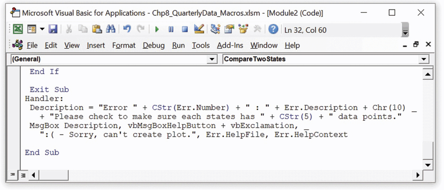
Vba Editing And Code Development Chapter 8 Excel Basics To Blackbelt from static.cambridge.org

You can read the full explanation in article how to count unique values in excel with multiple criteria? You can select the data you want in the chart and press alt + f1 to create a chart immediately, but it might not be the best chart for the data. To do this, you need only to create a table with multiple columns. Select chart and click on select data button. A simple chart in excel can say more than a sheet full of numbers. If i click on cell c22, to make it the active cell, then click on the autosum button in the editing group, the program will enter a formula into the cell. Select your data (both columns) and create a pivot table: Here you can choose which kind of chart should be created.

Select the fruit column you will create a chart based on, and press ctrl + c keys to copy.

Here, reduce the series overlap to 0. You should see a blank worksheet with grid lines. I can also use the editing group, on the home tab, to add up, count and find the averages of selections of number data. On a mac, you'll instead click the design tab, click add chart element, select chart title, click a location, and type in the graph's title. Add duration data to the chart. As you'll see, creating charts is very easy. Now that we have neighbor numbers and charts range (from step 1), we can create 7 named ranges, one per chart. In this article you will learn how to create a frequency analysis chart in excel. Click that rectangle (you may need to move or hide the text pane) and type the name of that person. Are the the neighbors to left. Select data for the chart. Excel has many types of charts that you can use depending on your needs. Remove the decimal digits and set the format code 0%.

If i click on cell c22, to make it the active cell, then click on the autosum button in the editing group, the program will enter a formula into the cell. This method will guide you to create a normal column chart by the count of values in excel. Use =index(charts, linked_cell_for_scrollbar) left1, left2, left3: However, if you can't use excel table for some reason (possibly if you are using excel 2003), there is another (slightly complicated) way to create dynamic chart ranges using excel formulas and named ranges. How to make a run chart in excel 1.

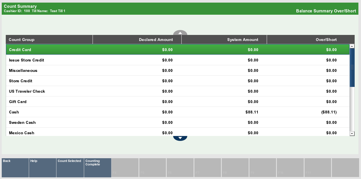
Register Open And Close from docs.oracle.com

To create a line chart, execute the following steps. However, if you can't use excel table for some reason (possibly if you are using excel 2003), there is another (slightly complicated) way to create dynamic chart ranges using excel formulas and named ranges. On the data tab, in the sort & filter group, click za. If i click on cell c22, to make it the active cell, then click on the autosum button in the editing group, the program will enter a formula into the cell. Click that rectangle (you may need to move or hide the text pane) and type the name of that person. Select your data (both columns) and create a pivot table: In the number subgroup change the common format on percentage. How to make a run chart in excel 1.

Now, let's use excel's replace feature to replace the 0 values in the example.

You can read the full explanation in article how to count unique values in excel with multiple criteria? Click on the series option. Are the the neighbors to left. Now select the pivot table data and create your pie chart as. When you select the chart, the ribbon activates the following tab. On the data tab, in the sort & filter group, click za. The two charts below are trying to show the same data. You will also learn how to create the number groups and how to show the % running total in the pivot table. Would you like to be able to show completed and not completed a. However, if you can't use excel table for some reason (possibly if you are using excel 2003), there is another (slightly complicated) way to create dynamic chart ranges using excel formulas and named ranges. If you don't have excel 2016 or later, simply create a pareto chart by combining a column chart and a line graph. A side bar will open in excel for the formatting of the chart. Select chart and click on select data button.